39 excel data labels from different column
Help: substitute x-axis label with data from different column This has been a challenge for me, but perhaps one of you knows better! I'm needing some graphing help and have attached a sample sheet. I have 3 columns: x: distance y: data z: sampling posts I've plotted distance vs data. However, instead of distance being the label for x-axis, I need the corresponding z-column (sampling posts) to be used instead. [SOLVED] Another column as data label? - Excel Help Forum Make a second series with same values but yr aliases as categories. Plot this new series on a second category axis. Effectively make the new bars completely invisible by selecting the attributes for fill and line to 'none'. Now select for the invisible series the data label and you shd get the desired effect.
Excel: Merge tables by matching column data or headers ... Oct 31, 2018 · The original tables are not changed. The data is combined into a new table that can be imported in an existing or a new worksheet. In Excel 2016 and Excel 2019, Power Query is an inbuilt feature. In Excel 2010 and Excel 2013, it can be downloaded as an add-in.

Excel data labels from different column
How to Print Labels from Excel Using Database Connections Open label design software. Click on Data Sources, and then click Create/Edit Query. Select Excel and name your database. Browse and attach your database file. Save your query so it can be used again in the future. Select the necessary fields (columns) that you would like to use on your label template. 😊. How to create Custom Data Labels in Excel Charts Add default data labels. Click on each unwanted label (using slow double click) and delete it. Select each item where you want the custom label one at a time. Press F2 to move focus to the Formula editing box. Type the equal to sign. Now click on the cell which contains the appropriate label. Press ENTER. How to Change Excel Chart Data Labels to Custom Values? May 05, 2010 · Now, click on any data label. This will select “all” data labels. Now click once again. At this point excel will select only one data label. Go to Formula bar, press = and point to the cell where the data label for that chart data point is defined. Repeat the process for all other data labels, one after another. See the screencast.
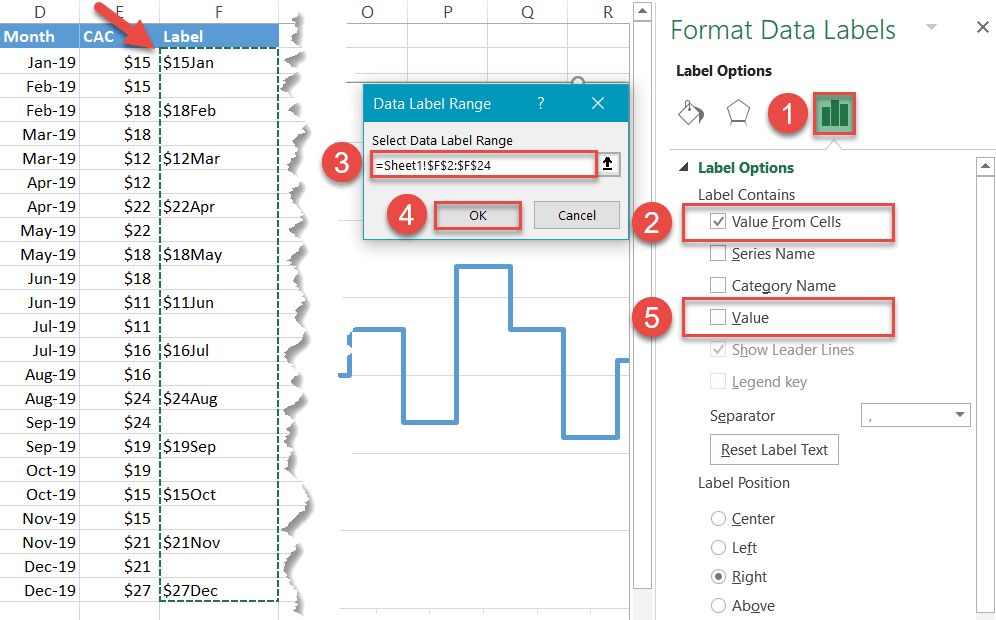
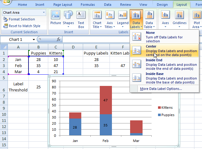
Excel data labels from different column. Move data labels - support.microsoft.com Click any data label once to select all of them, or double-click a specific data label you want to move. Right-click the selection > Chart Elements > Data Labels arrow, and select the placement option you want. Different options are available for different chart types. How do you label data points in Excel? - profitclaims.com This method will introduce a solution to add all data labels from a different column in an Excel chart at the same time. Please do as follows: 1. Right click the data series in the chart, and select Add Data Labels > Add Data Labels from the context menu to add data labels. 2. Using the CONCAT function to create custom data labels for an Excel ... Check the Value From Cells checkbox and select the cells containing the custom labels, cells C5 to C16 in this example. It is important to select the entire range because the label can move based on the data. Uncheck the Value checkbox because the value is incorporated in our custom label. The dialog box will look like this. Automatically copy data from different columns to certain column ... Those source sheets, however, are worrisome to me: In general I would recommend making them simpler and more functional, by which I mean, in part, place less emphasis on aesthetics (colors and separations) and more on just creating a clean table of data.
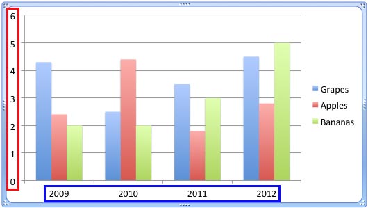
How to match and extract different columns in excel The dialog box will have changes. Highlight the 1 st three columns by clicking on the state column and the hold down the shift key, and click the infant mort. After that, click adds column button. The 1 st three columns will be copied to the output. You can copy other columns by holding down CTRL and clicking the columns. Understanding Excel Chart Data Series, Data Points, and Data Labels 19/09/2020 · Numeric Values: Taken from individual data points in the worksheet.; Series Names: Identifies the columns or rows of chart data in the worksheet. Series names are commonly used for column charts, bar charts, and line graphs. Category Names: Identifies the individual data points in a single series of data.These are commonly used for pie charts. Custom data labels in a chart - Get Digital Help Press with mouse on "Add Data Labels". Press with mouse on Add Data Labels". Double press with left mouse button on any data label to expand the "Format Data Series" pane. Enable checkbox "Value from cells". A small dialog box prompts for a cell range containing the values you want to use a s data labels. Select the cell range and press with ... How to Make Excel Clustered Stacked Column Chart - Data Fix Feb 01, 2022 · First year's data is in the left column; Second year's data is in the right column; Seasonal colours are similar, to make comparisons easier; 2b) Create a Clustered Stacked Bar Chart. If you chose the Stacked Bar chart type, the Clustered Stacked Bar chart should look like the one in the screenshot below. For each region:
Custom Data Labels with Colors and Symbols in Excel Charts - [How To] Step 4: Select the data in column C and hit Ctrl+1 to invoke format cell dialogue box. From left click custom and have your cursor in the type field and follow these steps: Press and Hold ALT key on the keyboard and on the Numpad hit 3 and 0 keys. Let go the ALT key and you will see that upward arrow is inserted. Adding labels to markers in Excel from a column in C# It allows for you to label with either the X, the Y, or both the X and Y values, but not with some categorical values. Create an array that contains the labels you want to apply. The array should be in the same order and contain as many labels as the series has points. Then, this is the method that I use in VBA: How can I add data labels from a third column to a scatterplot? Under Labels, click Data Labels, and then in the upper part of the list, click the data label type that you want. Under Labels, click Data Labels, and then in the lower part of the list, click where you want the data label to appear. Depending on the chart type, some options may not be available. Add or remove data labels in a chart - support.microsoft.com Right-click the data series or data label to display more data for, and then click Format Data Labels. Click Label Options and under Label Contains, select the Values From Cells checkbox. When the Data Label Range dialog box appears, go back to the spreadsheet and select the range for which you want the cell values to display as data labels.
microsoft excel - Cannot change column width or add separate data labels in date specific bar ...
Add Data Labels From Different Column In An Excel Chart A.docx Batch Add All Data Labels From Different Column In An Excel Chart This method will introduce a solution to add all data labels from a different column in an Excel chart at the same time. Please do as follows: 1 . Right click the data series in the chart, and select Add Data Labels > Add Data Labels from the context menu to add data labels. 2 .

excel - Column chart with primary and secondary y-axes - Stack Overflow
Dynamically Label Excel Chart Series Lines - My Online Training Hub To modify the axis so the Year and Month labels are nested; right-click the chart > Select Data > Edit the Horizontal (category) Axis Labels > change the 'Axis label range' to include column A. Step 2: Clever Formula The Label Series Data contains a formula that only returns the value for the last row of data.

How to Make a Bar Graph In Excel | HowStuffWorks
Understanding Excel Chart Data Series, Data Points, and Data ... Sep 19, 2020 · Numeric Values: Taken from individual data points in the worksheet.; Series Names: Identifies the columns or rows of chart data in the worksheet. Series names are commonly used for column charts, bar charts, and line graphs.
Changing Axis Labels in PowerPoint 2011 for Mac
Create Dynamic Chart Data Labels with Slicers - Excel Campus You basically need to select a label series, then press the Value from Cells button in the Format Data Labels menu. Then select the range that contains the metrics for that series. Click to Enlarge Repeat this step for each series in the chart. If you are using Excel 2010 or earlier the chart will look like the following when you open the file.
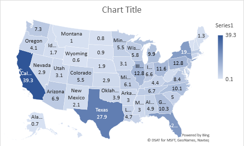
Excel map chart
Two Variable Data Table in Excel | How to Perform Two Variable … Step 7: Data Table pop up will appear with two input cells for the row, and column >Select Loan amount in the Row input cell and interest rate in Column input cell > click ok button. Step 8: Result will be published per month loan re-payment amount as per the combination of different Interest rate and loan amount data set.
How to Create a Step Chart in Excel - Automate Excel
Apply Custom Data Labels to Charted Points - Peltier Tech Select an individual label (two single clicks as shown above, so the label is selected but the cursor is not in the label text), type an equals sign in the formula bar, click on the cell containing the label you want, and press Enter. The formula bar shows the link (=Sheet1!$D$3). Repeat for each of the labels.

Excel Pivot Table Tutorial & Sample | Productivity Portfolio
How to Use Cell Values for Excel Chart Labels Select range A1:B6 and click Insert > Insert Column or Bar Chart > Clustered Column. The column chart will appear. We want to add data labels to show the change in value for each product compared to last month. Advertisement Select the chart, choose the "Chart Elements" option, click the "Data Labels" arrow, and then "More Options."

How to Create Multi-Category Chart in Excel - Excel Board
How to Customize Your Excel Pivot Chart Data Labels - dummies To remove the labels, select the None command. If you want to specify what Excel should use for the data label, choose the More Data Labels Options command from the Data Labels menu. Excel displays the Format Data Labels pane. Check the box that corresponds to the bit of pivot table or Excel table information that you want to use as the label.
How to Add Data Labels in Excel - Excelchat | Excelchat
How to Print Labels From Excel - EDUCBA Step #1 - Add Data into Excel Create a new excel file with the name "Print Labels from Excel" and open it. Add the details to that sheet. As we want to create mailing labels, make sure each column is dedicated to each label. Ex.
Excel Dashboard Templates How-to Make Conditional Label Values in an Excel Stacked Column Chart ...
Use the Column Header to Retrieve Values from an Excel Table This post discusses ways to retrieve aggregated values from a table based on the column labels. Overview. Beginning with Excel 2007, we can store data in a table with the Insert > Table Ribbon command icon. If you haven't yet explored this incredible feature, please check out this CalCPA Magazine article Excel Rules.. Frequently, we need to retrieve values out of data tables for reporting or ...

30 How To Label Columns In Excel 2016 - Labels Database 2020
How to Print Labels from Excel - Lifewire Select Mailings > Write & Insert Fields > Update Labels . Once you have the Excel spreadsheet and the Word document set up, you can merge the information and print your labels. Click Finish & Merge in the Finish group on the Mailings tab. Click Edit Individual Documents to preview how your printed labels will appear. Select All > OK .

How to Create a MS Excel Pivot Table – An Introduction | SIMPLE TAX INDIA
One Variable Data Table in Excel | Step by Step Tutorials One Variable Data Table in Excel allows users to test how one variable or value in a data table affects the result in the created formula. It is only useful when the formula depends on several values that can be used for one variable. For the complete data table, we can test only one single input cell for a series of values on the basis of the What-If analysis option, which is available …

Charting in Excel - Adding Data Labels - YouTube
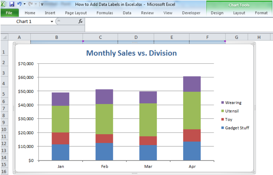
How to Add Total Data Labels to the Excel Stacked Bar Chart Apr 03, 2013 · Step 4: Right click your new line chart and select “Add Data Labels” Step 5: Right click your new data labels and format them so that their label position is “Above”; also make the labels bold and increase the font size. Step 6: Right click the line, select “Format Data Series”; in the Line Color menu, select “No line”
Sales Analysis Charts in Excel - 78 Alternatives
Column Chart with Category Axis Labels Between Columns Click the menu key (between the right Alt and Ctrl buttons on most Windows keyboards) or hold Shift and click the F10 function key to pop up the context menu. Click Change Series Chart Type, and choose XY Scatter. This adds a set of markers along the bottom of the chart (I used blue circles in the chart below) and it adds secondary X and Y axes.
Creating a chart with dynamic labels - Microsoft Excel 2013
Create a multi-level category chart in Excel - ExtendOffice Select the dots, click the Chart Elements button, and then check the Data Labels box. 23. Right click the data labels and select Format Data Labels from the right-clicking menu. 24. In the Format Data Labels pane, please do as follows. 24.1) Check the Value From Cells box;
Post a Comment for "39 excel data labels from different column"