45 how to display data labels in excel chart
How to Add Labels to Scatterplot Points in Excel - Statology Next, click anywhere on the chart until a green plus (+) sign appears in the top right corner. Then click Data Labels, then click More Options… In the Format Data Labels window that appears on the right of the screen, uncheck the box next to Y Value and check the box next to Value From Cells. How To Create Labels In Excel Blindatthemuseum Click edit individual documents to preview how your printed labels will appear. Select the chart label you want to change. Right click the data series in the chart, and select add data labels > add data labels from the context menu to add data labels. Click The Create Cards Icon In The Transform Group On The Ablebits Tools Tab:
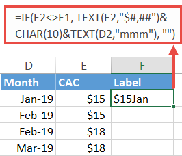
Custom Chart Data Labels In Excel With Formulas Follow the steps below to create the custom data labels. Select the chart label you want to change. In the formula-bar hit = (equals), select the cell reference containing your chart label's data. In this case, the first label is in cell E2. Finally, repeat for all your chart laebls.
How to display data labels in excel chart
How To Add Data Labels In Excel - ashokasouthside.info Then, click the insert tab along the top ribbon and click the insert scatter (x,y) option in the charts group. Click on the arrow next to data labels to change the position of where the labels are in relation to the bar chart. To format data labels in excel, choose the set of data labels to format. Source: Displaying Data in a Chart with ASP.NET Web Pages (Razor) When you want to display your data in graphical form, you can use Chart helper. The Chart helper can render an image that displays data in a variety of chart types. It supports many options for formatting and labeling. support.microsoft.com › en-us › officeAdd or remove data labels in a chart - support.microsoft.com When the Data Label Range dialog box appears, go back to the spreadsheet and select the range for which you want the cell values to display as data labels. When you do that, the selected range will appear in the Data Label Range dialog box. Then click OK. The cell values will now display as data labels in your chart.
How to display data labels in excel chart. 6 Tips for Making Microsoft Excel Charts That Stand Out Select the Right Chart for the Data. The first step in creating a chart or graph is selecting the one that best fits your data. You can gain a lot of insight on this by looking at Excel's suggestions. Select the data you want to plot on a chart. Then, head to the Insert tab and Charts section of the ribbon. Format Data Labels in Excel- Instructions - TeachUcomp, Inc. 14/11/2019 · Format Data Labels in Excel: Instructions. To format data labels in Excel, choose the set of data labels to format. One way to do this is to click the “Format” tab within the “Chart Tools” contextual tab in the Ribbon. Then select the data labels to format from the “Current Selection” button group. How to Show Percentage in Pie Chart in Excel? - GeeksforGeeks Show percentage in a pie chart: The steps are as follows : Select the pie chart. Right-click on it. A pop-down menu will appear. Click on the Format Data Labels option. The Format Data Labels dialog box will appear. In this dialog box check the "Percentage" button and uncheck the Value button. This will replace the data labels in pie chart ... How to Create and Customize a Treemap Chart in Microsoft Excel Select the data for the chart and head to the Insert tab. Click the "Hierarchy" drop-down arrow and select "Treemap." The chart will immediately display in your spreadsheet. And you can see how the rectangles are grouped within their categories along with how the sizes are determined.
Add or remove data labels in a chart - support.microsoft.com When the Data Label Range dialog box appears, go back to the spreadsheet and select the range for which you want the cell values to display as data labels. When you do that, the selected range will appear in the Data Label Range dialog box.Then click OK.. The cell values will now display as data labels in your chart. How to Create a Waterfall Chart in Excel - SpreadsheetDaddy Let's see how to do it! 1. Click on your chart. 2. Navigate to the Design tab. 3. Choose Add Chart Element. 4. Click Data Labels. 5. Select the label position: Center, Inside End, Inside Base, Outside End, or Data Callout — whatever works best for your chart. How to Apply a Different Style to Your Waterfall Chart in Excel How to Add Axis Titles in a Microsoft Excel Chart Select your chart and then head to the Chart Design tab that displays. Click the Add Chart Element drop-down arrow and move your cursor to Axis Titles. In the pop-out menu, select "Primary Horizontal," "Primary Vertical," or both. If you're using Excel on Windows, you can also use the Chart Elements icon on the right of the chart. How to add data labels from different column in an Excel chart? This method will guide you to manually add a data label from a cell of different column at a time in an Excel chart. 1.Right click the data series in the chart, and select Add Data Labels > Add Data Labels from the context menu to add data labels.. 2.
Text Labels on a Horizontal Bar Chart in Excel - Peltier Tech 21/12/2010 · When analyzing survey results, for example, there may be a numerical scale that has associated text labels. This may be a scale of 1 to 5 where 1 means “Completely Dissatisfied” and 5 means “Completely Satisfied”, with other labels in between. The data can be plotted by value, but it’s not obvious how to place […] DataLabels.ShowValue property (Excel) | Microsoft Docs This example enables the value to be shown for the data labels of the first series, on the first chart. This example assumes that a chart exists on the active worksheet. VB Copy Sub UseValue () ActiveSheet.ChartObjects (1).Activate ActiveChart.SeriesCollection (1) _ .DataLabels.ShowValue = True End Sub Support and feedback Format Chart Axis in Excel - Axis Options However, In this blog, we will be working with Axis options, Tick marks, Labels, Number > Axis options> Axis options> Format Axis Pane. Axis Options: Axis Options There are multiple options So we will perform one by one. Changing Maximum and Minimum Bounds The first option is to adjust the maximum and minimum bounds for the axis. Understanding Excel Chart Data Series, Data Points, and Data Labels 19/09/2020 · Numeric Values: Taken from individual data points in the worksheet.; Series Names: Identifies the columns or rows of chart data in the worksheet. Series names are commonly used for column charts, bar charts, and line graphs. Category Names: Identifies the individual data points in a single series of data.These are commonly used for pie charts.
34 Label Data Points In Excel - Best Labels Ideas 2020
excel - How to not display labels in pie chart that are 0% - Stack Overflow Generate a new column with the following formula: =IF (B2=0,"",A2) Then right click on the labels and choose "Format Data Labels". Check "Value From Cells", choosing the column with the formula and percentage of the Label Options. Under Label Options -> Number -> Category, choose "Custom". Under Format Code, enter the following:
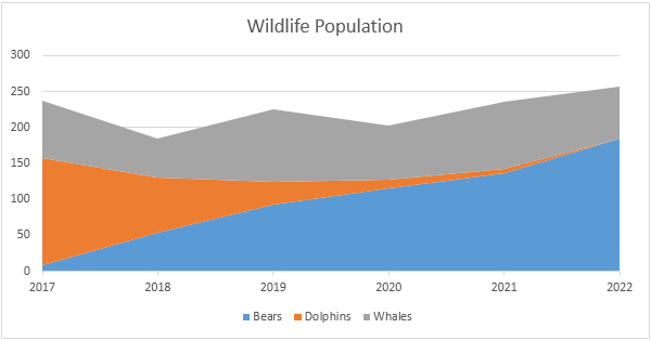
Area Chart in Excel - Easy Excel Tutorial
How to Apply a Filter to a Chart in Microsoft Excel Select the chart and you'll see buttons display to the right. Click the Chart Filters button (funnel icon). When the filter box opens, select the Values tab at the top. You can then expand and filter by Series, Categories, or both. Simply check the options you want to view on the chart, then click "Apply."
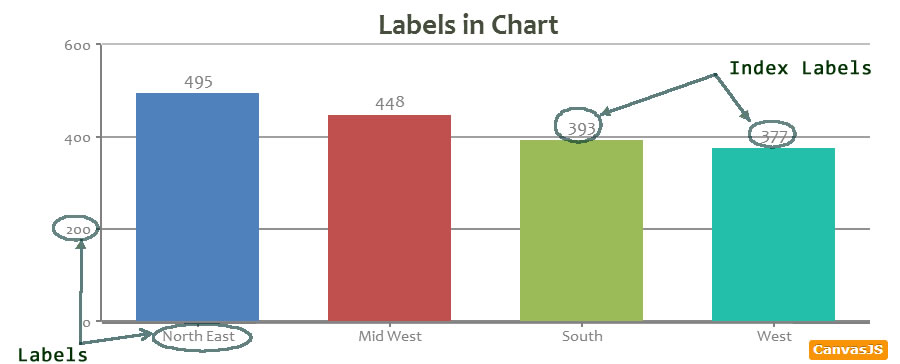
Tutorial on Labels & Index Labels in Chart | CanvasJS JavaScript Charts
How to Add Custom Error Bars in Excel (2 Examples) STEPS: Firstly, select the averages to plot those averages in the bar chart. So, we select cell B11:E11. Secondly, go to the Insert tab from the ribbon. Thirdly, in the Charts category, click on the Insert Column or Bar Chart drop-down menu and choose the first chart, Clustered Column from the 2-D Column.
How to Create a Step Chart in Excel - Automate Excel
support.microsoft.com › en-us › officeEdit titles or data labels in a chart - support.microsoft.com To reposition all data labels for an entire data series, click a data label once to select the data series. To reposition a specific data label, click that data label twice to select it. This displays the Chart Tools , adding the Design , Layout , and Format tabs.

Excel 2013 Tutorial Formatting Data Labels Microsoft Training Lesson 28.6 - YouTube
DataLabel object (Excel) | Microsoft Docs With Charts ("chart1") With .SeriesCollection (1).Points (2) .HasDataLabel = True .DataLabel.Text = "Saturday" End With End With On a trendline, the DataLabel property returns the text shown with the trendline. This can be the equation, the R-squared value, or both (if both are showing).
Panel Bar Chart in Excel with 3 sets of data - XcelanZ
How to Change Excel Chart Data Labels to Custom Values? 05/05/2010 · Now, click on any data label. This will select “all” data labels. Now click once again. At this point excel will select only one data label. Go to Formula bar, press = and point to the cell where the data label for that chart data point is defined. Repeat the process for all other data labels, one after another. See the screencast.

How to Make Excel Charts More Intuitive by Adding Data Labels and Tables - Data Recovery Blog
› documents › excelHow to display text labels in the X-axis of scatter chart in ... Actually, there is no way that can display text labels in the X-axis of scatter chart in Excel, but we can create a line chart and make it look like a scatter chart. 1. Select the data you use, and click Insert > Insert Line & Area Chart > Line with Markers to select a line chart. See screenshot: 2. Then right click on the line in the chart to ...

Enable or Disable Excel Data Labels at the click of a button - How To - PakAccountants.com
Create Dynamic Chart Data Labels with Slicers - Excel Campus 10/02/2016 · Typically a chart will display data labels based on the underlying source data for the chart. In Excel 2013 a new feature called “Value from Cells” was introduced. This feature allows us to specify the a range that we want to use for the labels. Since our data labels will change between a currency ($) and percentage (%) formats, we need a ...

How to Create a Chart in Microsoft Excel - TechSupport
How to Show Percentages in Stacked Column Chart in Excel? Implementation: Follow the below steps to show percentages in stacked column chart In Excel: Step 2: Select the entire data table. Step 3: To create a column chart in excel for your data table. Go to "Insert" >> "Column or Bar Chart" >> Select Stacked Column Chart. Step 4: Add Data labels to the chart. Goto "Chart Design" >> "Add ...

How to Add Data Labels to an Excel 2010 Chart - dummies
5 New Charts to Visually Display Data in Excel 2019 - dummies Place text labels describing the data sets above the data. Select the data sets and their column labels. Click Insert → Insert Statistic Chart → Box and Whisker. Format the chart as desired. Box and whisker charts are visually similar to stock price charts, which Excel can also create, but the meaning is very different.
Displaying Numbers in Thousands in a Chart in Microsoft Excel | Microsoft Excel Tips from Excel ...
Chart.ApplyDataLabels method (Excel) | Microsoft Docs Syntax expression. ApplyDataLabels ( Type, LegendKey, AutoText, HasLeaderLines, ShowSeriesName, ShowCategoryName, ShowValue, ShowPercentage, ShowBubbleSize, Separator) expression A variable that represents a Chart object. Parameters Example This example applies category labels to series one on Chart1. VB Copy Charts ("Chart1").SeriesCollection (1).

Excel Charts Archives - PakAccountants.com
Modifying Axis Scale Labels (Microsoft Excel) Follow these steps: Create your chart as you normally would. Double-click the axis you want to scale. You should see the Format Axis dialog box. (If double-clicking doesn't work, right-click the axis and choose Format Axis from the resulting Context menu.) Make sure the Number tab is displayed. (See Figure 1.)

» Excel Charts: Creating Custom Data Labels
How To Show Two Sets of Data on One Graph in Excel To do so, click and drag your mouse across all the data you want, including the names of the columns and rows. You can check that you selected the data by looking for the cells to be gray instead of white. 3. Click the "Insert" tab and then look at the "Recommended Charts" in the charts group

Format Number Options for Chart Data Labels in PowerPoint 2011 for Mac
Excel Map Chart not showing DATA LABELS for all INDIAN PROVINCES Excel Map Chart not showing DATA LABELS for all INDIAN PROVINCES. I've previously posted regarding issues (bugs) with the way the Excel Map chart feature works. I've been putting country risk charts together for a client and I'd like present the data in a map chart. I've found that sometimes it works and sometimes it doesn't requiring you to ...
Adding data labels to see the value of the bars in an Excel chart
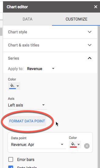
How to: Display and Format Data Labels - DevExpress To display value labels, set the DataLabelBase.ShowValue property of the DataLabelOptions object to true. Series name. Series labels identify data series to which the data points in the chart belong. Most series include multiple data points, so the same name will be repeated for all data points in the series, which is probably overkill.

How-to Display Metrics Data in an Excel Dashboard Chart - YouTube
How to Display Percentage in an Excel Graph (3 Methods) Then go to the More Options via the right arrow beside the Data Labels. Select Chart on the Format Data Labels dialog box. Uncheck the Value option. Check the Value From Cells option. Then you have to select cell ranges to extract percentage values. For this purpose, create a column called Percentage using the following formula: =E5/C5
Post a Comment for "45 how to display data labels in excel chart"