40 pivot table concatenate row labels

Pivot Table calendar - Get Digital Help Apr 15, 2020 · Insert Pivot Table. A Pivot Table is a feature in Excel that is perhaps the most powerful of all features but also least known. It allows you to quickly summarize and analyze data, it is incredibly fast and easy to work with. The image above shows an empty Pivot Table placed on a worksheet, the task pane to the right allows you to quickly configure the Pivot Table. Create Regular Excel Charts from PivotTables - My Online … May 22, 2020 · 1 Pivot Manual Table 2 Row Labels Revenue Profit GM% Year Revenue Profit GM% 3 2018 $19,807,854 $10,212,533 59% 2018 #REF! ... but I solved the problem. I needed to Concatenate the Year value into the GETPIVOTDATA formula like this: ... I followed the steps and was able to create a regular chart off my pivot table using Dynamic Named Ranges. ...

How to make and use Pivot Table in Excel - Ablebits.com Sep 30, 2022 · It might be useful to create a Pivot Table and Pivot Chart at the same time. To do this, in Excel 2013 and higher, go to the Insert tab > Charts group, click the arrow below the PivotChart button, and then click PivotChart & PivotTable. In Excel 2010 and 2007, click the arrow below PivotTable, and then click PivotChart.

Pivot table concatenate row labels

How to Change Excel Chart Data Labels to Custom Values? - Chandoo.org May 05, 2010 · Col B is all null except for “1” in each cell next to the labels, as a helper series, iaw a web forum fix. Col A is x axis labels (hard coded, no spaces in strings, text format), with null cells in between. The labels are every 4 or 5 rows apart with null in between, marking month ends, the data columns are readings taken each week. › Advanced-pivot-table-techniques6 Advanced Pivot Table Techniques You Should Know in 2022 1. While clicked inside a cell of the pivot table, visit the “Pivot Table Analyze” tab of the ribbon, select the button for “Fields, Items, and Sets,” and then click on “Calculated Field.” 2. In the popup, enter the name of the new calculated field (in this case, Jason would name it “profit” or something similar). 3. › Excel › ResourcesExcel Pivot Table Tutorial - 5 Easy Steps for Beginners 2. Insert pivot table. Believe it or not, we’re already to the point in the process when you can insert a pivot table into your workbook. To do so, highlight your entire data set (including the column headers), click “Insert” on the ribbon, and then click the “Pivot Table” button. 3. Choose where to place your pivot table

Pivot table concatenate row labels. Text Manipulation Formulas in Excel - Vertex42.com Nov 29, 2017 · 3. Concatenate a text string. You can use CONCATENATE, the & operator, or the newer CONCAT and TEXTJOIN functions to concatenate strings. The following formulas combine a first name in cell A1 and a last name in cell B1 with a space in the middle. The result is "John Smith" for all four formulas. Sharing Tips and Tutorials for Excel - ExtendOffice Reuse Anything: Add the most used or complex formulas, charts and anything else to your favorites, and quickly reuse them in the future. More than 20 text features: Extract Number from Text String; Extract or Remove Part of Texts; Convert Numbers and Currencies to English Words. Merge Tools: Multiple Workbooks and Sheets into One; Merge Multiple Cells/Rows/Columns … Excel Pivot Table Tutorial - 5 Easy Steps for Beginners - GoSkills… 2. Insert pivot table. Believe it or not, we’re already to the point in the process when you can insert a pivot table into your workbook. To do so, highlight your entire data set (including the column headers), click “Insert” on the ribbon, and then click the “Pivot Table” button. 3. Choose where to place your pivot table 6 Advanced Pivot Table Techniques You Should Know in 2022 1. While clicked inside a cell of the pivot table, visit the “Pivot Table Analyze” tab of the ribbon, select the button for “Fields, Items, and Sets,” and then click on “Calculated Field.” 2. In the popup, enter the name of the new calculated field (in this case, Jason would name it “profit” or something similar). 3.

› pivot-table-calendarPivot Table calendar - Get Digital Help Apr 15, 2020 · The image above shows an empty Pivot Table placed on a worksheet, the task pane to the right allows you to quickly configure the Pivot Table. The task pane appears automatically when you select any cell in the Pivot Table and disappears when you go outside the Pivot Table. Go to a new sheet, I named it "Calendar". Go to tab "Insert" on the ribbon. › documents › excelSharing Tips and Tutorials for Excel - ExtendOffice How to make row labels on same line in pivot table? How to make sheet tab name equal to cell value in Excel? How to make specific cells unselectable in Excel? How to make the background color of checkbox transparent in Excel? How to make the worksheet very hidden and visible in Excel? How to make top row always stay visible in Excel? chandoo.org › wp › change-data-labels-in-chartsHow to Change Excel Chart Data Labels to Custom Values? May 05, 2010 · Col B is all null except for “1” in each cell next to the labels, as a helper series, iaw a web forum fix. Col A is x axis labels (hard coded, no spaces in strings, text format), with null cells in between. The labels are every 4 or 5 rows apart with null in between, marking month ends, the data columns are readings taken each week. techcommunity.microsoft.com › t5 › excelMatch names between two sheets and return value of a cell in ... Dec 19, 2017 · So in sheet 2 if a site name in coulomb B matches a site name in sheet 1 coulomb A, return the value from a specific cell in the same row as where the names matched. The data is sorted on dates which may change and I need to be able to show the updated date value in sheet 2 when date and order changes in sheet 1 for a specific site name.

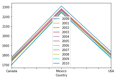
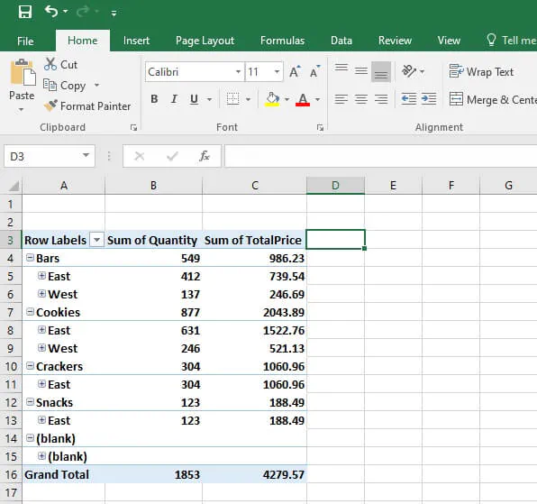
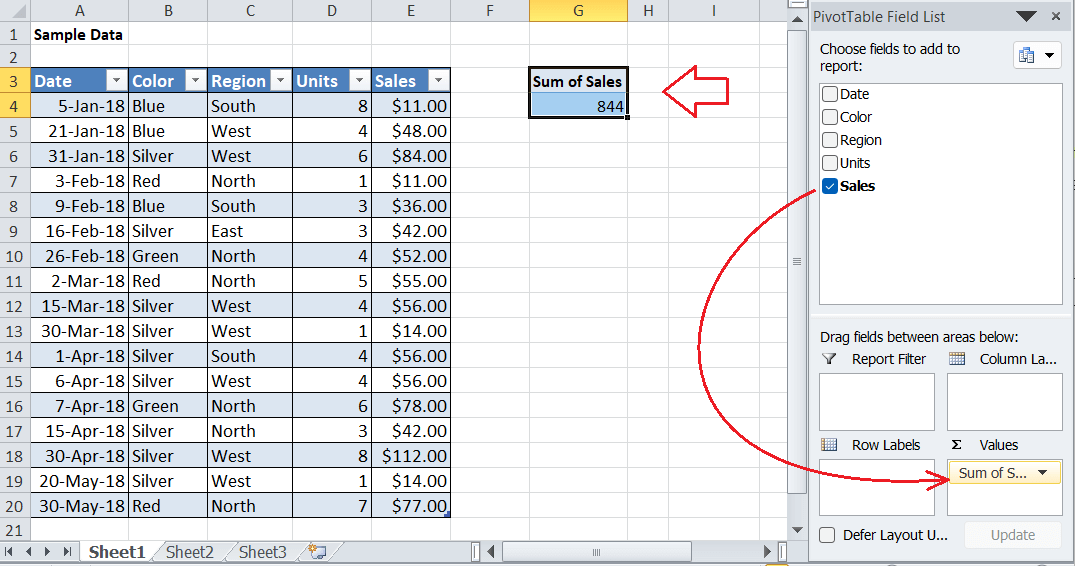
Count Unique Items in Pivot Table - Contextures Excel Tips May 11, 2022 · To create the pivot table, try the following steps: Select a cell in the source data table. At the bottom of the Create PivotTable dialog box, add a check mark to "Add this data to the Data Model" Click the OK button; Add Fields to Pivot Table. Next, to set up the pivot table layout, follow these steps: In the pivot table, add Region to the Row ... › create-regular-excelCreate Regular Excel Charts from PivotTables • My Online ... May 22, 2020 · How to Create Regular Excel Charts from PivotTables Method 1: Manual Chart Table. A while ago I showed you how to create Excel charts from Multiple PivotTables.And this is great if your data needs arranging into contiguous cells so it can be plotted as one series, or if the source data is inconsistent in the two PivotTables and needs organising first. Match names between two sheets and return value of a cell in the row Dec 19, 2017 · Hi . I am looking for a way to match a name between two sheets and then return a date value which is in a different cell in the same row. So in sheet 2 if a site name in coulomb B matches a site name in sheet 1 coulomb A, return the value from a specific cell in the same row as where the names matched. › Excel › ResourcesExcel Pivot Table Tutorial - 5 Easy Steps for Beginners 2. Insert pivot table. Believe it or not, we’re already to the point in the process when you can insert a pivot table into your workbook. To do so, highlight your entire data set (including the column headers), click “Insert” on the ribbon, and then click the “Pivot Table” button. 3. Choose where to place your pivot table

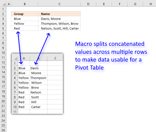
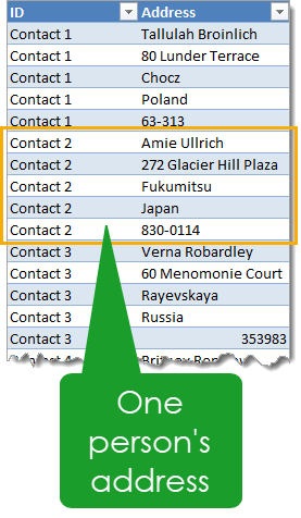
Prepare data for Pivot Table – How to split concatenated values?

› Advanced-pivot-table-techniques6 Advanced Pivot Table Techniques You Should Know in 2022 1. While clicked inside a cell of the pivot table, visit the “Pivot Table Analyze” tab of the ribbon, select the button for “Fields, Items, and Sets,” and then click on “Calculated Field.” 2. In the popup, enter the name of the new calculated field (in this case, Jason would name it “profit” or something similar). 3.

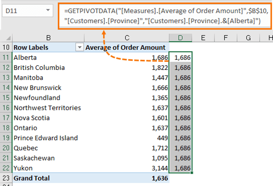
GETPIVOTDATA Function for Power Pivot • My Online Training Hub

How to Change Excel Chart Data Labels to Custom Values? - Chandoo.org May 05, 2010 · Col B is all null except for “1” in each cell next to the labels, as a helper series, iaw a web forum fix. Col A is x axis labels (hard coded, no spaces in strings, text format), with null cells in between. The labels are every 4 or 5 rows apart with null in between, marking month ends, the data columns are readings taken each week.

5 Ways to Concatenate Data with a Line Break in Excel | How ...

Solved: Pivot table with multiple sub groups in both rows ...

Pivot Table Filter in Excel | How to Filter Data in a Pivot ...

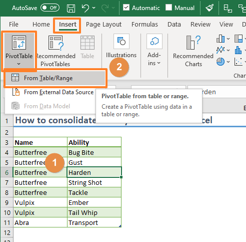
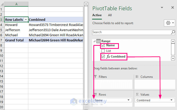
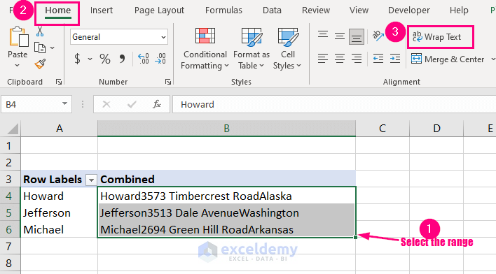
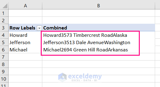
How to consolidate text with Pivot Table in Excel

Concatenation (Combining Data Tables) in Python and Pandas: A ...

Excel: Reporting Text in a Pivot Table - Strategic Finance

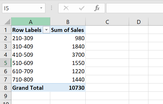
How to Make a Histogram with Pivot Table – TutorialsForExcel

Solved: Concatenate rows values - Microsoft Power BI Community

How to Use CONCATENATE Function in Excel [Step-by-Step]

Show Text in a Pivot Table Values Area | Excel Pivot Tables

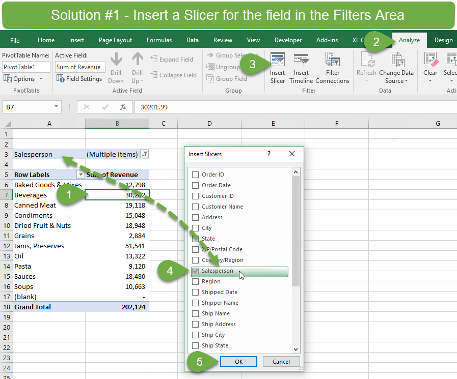
3 Ways to Display (Multiple Items) Filter Criteria in a Pivot ...

Pivot Tables Excel 2007: Combine rows/ columns to create a ...

How to add a percentage column in a pivot table. - ITFixed ...

Solved: Table Transformer - concatenate data from multiple...

Merge two relational data sets

How to Add New Line with CONCATENATE Formula in Excel (5 Ways)

Merge, join, and concatenate — pandas 0.18.0 documentation

6 Advanced Pivot Table Techniques You Should Know in 2022

6 Advanced Pivot Table Techniques You Should Know in 2022

Pivot Table Filter | How to Filter Data in Pivot Table with ...

How to make and use Pivot Table in Excel

Pivot Table With Text in Values Area - Excel Tips - MrExcel ...

How to Add New Line with CONCATENATE Formula in Excel (5 Ways)

How to Create Pivot Table Calculated Fields | GoSkills

Merge, join, concatenate and compare — pandas 1.5.0 documentation

Excel: Reporting Text in a Pivot Table - Strategic Finance

How to consolidate text with Pivot Table in Excel

How to Add New Line with CONCATENATE Formula in Excel (5 Ways)

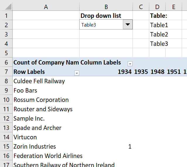
Change PivotTable data source using a drop-down list

Pivot Tables Some Useful Functions Insert Function Paste Special

How to consolidate text with Pivot Table in Excel

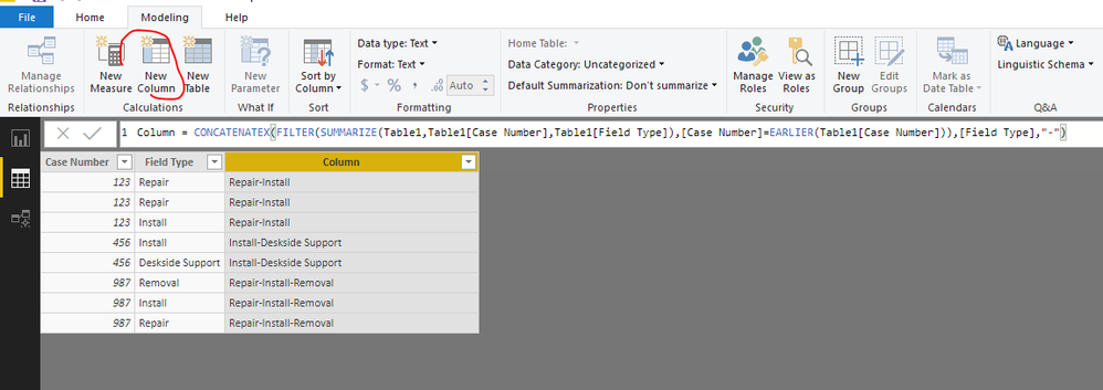
Concatenate multiple row values into one based on ...

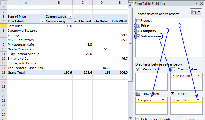
How can I concatenate values of Pivot Table columns in Excel ...

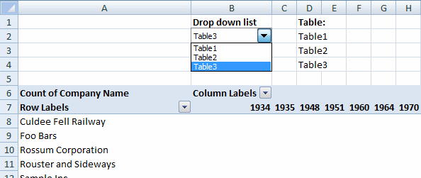
Change PivotTable data source using a drop-down list

How to Repeat Row Labels in a Pivot Table - Question and ...

Excel: Reporting Text in a Pivot Table - Strategic Finance

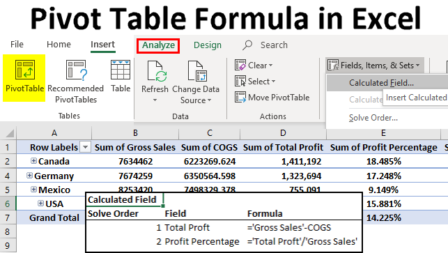
Pivot Table Formula in Excel | Steps to Use Pivot Table ...

How to create a Pivot Table in excel - javatpoint

Share :