44 excel 2013 data labels

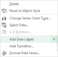
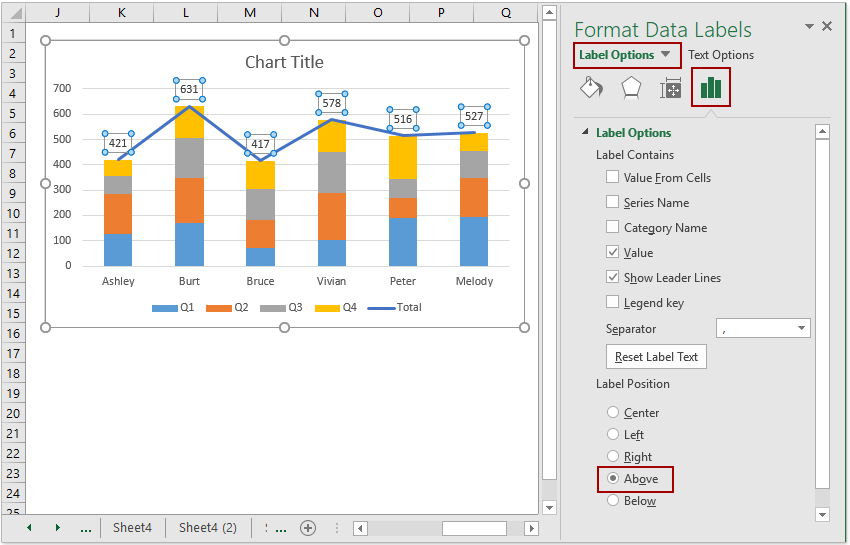
Adding Data Labels to Your Chart - Excel ribbon tips Select the position that best fits where you want your labels to appear. To add data labels in Excel 2013 or later versions, follow these steps: Activate the chart by clicking on it, if necessary. Make sure the Design tab of the ribbon is displayed. (This will appear when the chart is selected.) Click the Add Chart Element drop-down list. 4 steps: How to Create Waterfall Charts in Excel 2013 Select the primary vertical axis (y-axis) and delete as well. Add a chart title -in this case " FY15 Free Cash Flow ". Add data labels by right-clicking one of the series and selecting "Add data labels…". Add labels to each of the series apart from the invisible column. Select the data labels and make them bold, change colour as ...

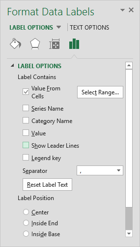
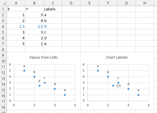
Excel Data Labels - Value from Cells To automatically update titles or data labels with changes that you make on the worksheet, you must reestablish the link between the titles or data labels and the corresponding worksheet cells. For data labels, you can reestablish a link one data series at a time, or for all data series at the same time.

Excel 2013 data labels

How to Customize Chart Elements in Excel 2013 - dummies To add data labels to your selected chart and position them, click the Chart Elements button next to the chart and then select the Data Labels check box before you select one of the following options on its continuation menu: Center to position the data labels in the middle of each data point, Excel 2013 Graphs automatically aligning data labels to end of bar Excel 2013 Graphs automatically aligning data labels to end of bar, Hi, In Excel 2013 I am wanting to align the data labels in a graph automatically to be at the end of the bar (in a bar graph obviously). I know how to move them manually, but I remember there used to be a way to make it move them all automatically. Data Labels in Excel Pivot Chart (Detailed Analysis) 7 Suitable Examples with Data Labels in Excel Pivot Chart Considering All Factors, 1. Adding Data Labels in Pivot Chart, 2. Set Cell Values as Data Labels, 3. Showing Percentages as Data Labels, 4. Changing Appearance of Pivot Chart Labels, 5. Changing Background of Data Labels, 6. Dynamic Pivot Chart Data Labels with Slicers, 7.

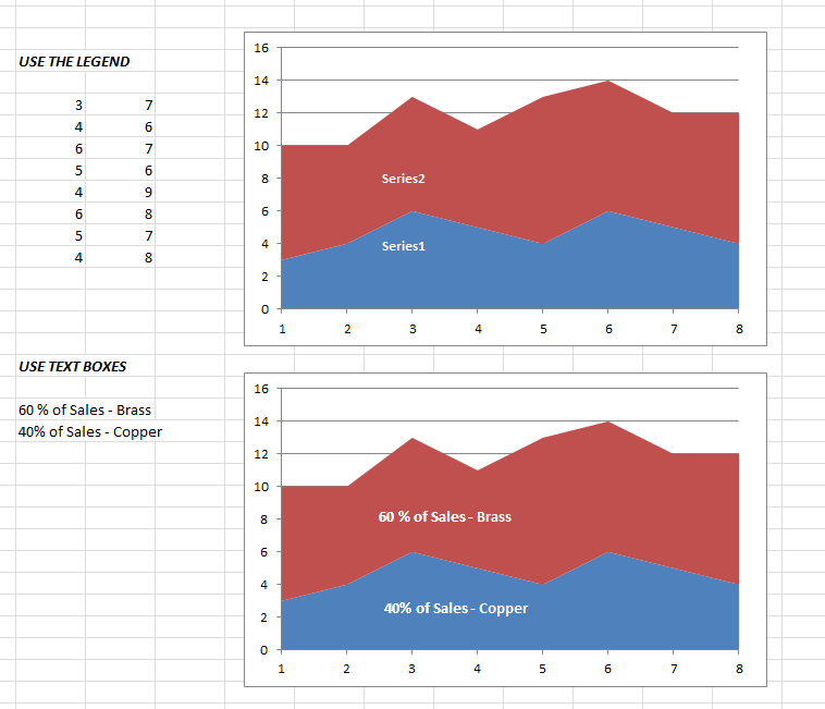
Excel 2013 data labels. How to Print Labels from Excel - Lifewire To label legends in Excel, select a blank area of the chart. In the upper-right, select the Plus ( +) > check the Legend checkbox. Then, select the cell containing the legend and enter a new name. How do I label a series in Excel? To label a series in Excel, right-click the chart with data series > Select Data. How to Add Data Tables to Charts in Excel 2013 - dummies To add a data table to your selected chart and position and format it, click the Chart Elements button next to the chart and then select the Data Table check box before you select one of the following options on its continuation menu: With Legend Keys to have Excel draw the table at the bottom of the chart, including the color keys used in the ... How To Add Data Labels In Excel - tequis.info You Can Easily Show Two Parameters In The Data Label. In excel 2013 or 2016. Select mailings > write & insert fields > update labels. Click on the arrow next to data labels to change the position of where the labels are in relation to the bar chart. Add A Label (Form Control) Click Developer, Click Insert, And Then Click Label. ... Values From Cell: Missing Data Labels Option in Excel 2013? When a chart created in 2013 using the "Values from Cell" data label option is opened with any earlier version of Excel, the data labels will show as " [CELLRANGE]". If you want to ensure that data labels survive different generations of Excel, you need to revert to the old technique: Insert data labels, Edit each individual data label,

"Chart created in Excel 2013 is now showing data label values when ... Hello everybody, 1) I created a customized column chart in Excel (A->G/57->83): The data labels show "Name" "%fraction" "(absolute share)" 2) The data of this chart is in the same excel sheet - but "far away" from the chart (AG->AV/444->454) 3) The chart is connected with the data by the "Value from cells" option: If you "right click2 on one of the data labels of the chart -> Click "Format ... Excel 2013 Chart Labels don't appear properly - Microsoft Community You've stumbled on a big problem - Excel 2013 lets you edit data labels directly, but this feature (rich text data labels) is not backwards-compatible and there's no way to turn it off. It's great to be able to modify the text of labels, or direct them to get contents from a worksheet cell. How to add data labels from different column in an Excel chart? Right click the data series, and select Format Data Labels from the context menu. 3. In the Format Data Labels pane, under Label Options tab, check the Value From Cells option, select the specified column in the popping out dialog, and click the OK button. Now the cell values are added before original data labels in bulk. 4. Custom Chart Data Labels In Excel With Formulas - How To Excel At Excel Select the chart label you want to change. In the formula-bar hit = (equals), select the cell reference containing your chart label's data. In this case, the first label is in cell E2. Finally, repeat for all your chart laebls. If you are looking for a way to add custom data labels on your Excel chart, then this blog post is perfect for you.

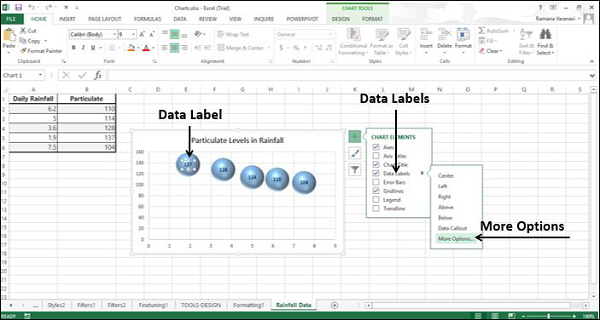
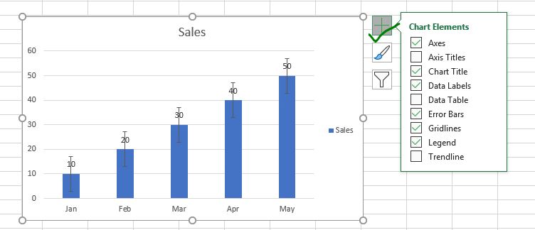
Excel charts: add title, customize chart axis, legend and data labels Add title to chart in Excel. In Excel 2013 - 365, a chart is already inserted with the default "Chart Title". To change the title text, simply select that box and type your title: ... Adding data labels to Excel charts. To make your Excel graph easier to understand, you can add data labels to display details about the data series. ... Quick Tip: Excel 2013 offers flexible data labels | TechRepublic right-click and choose Insert Data Label Field. In the next dialog, select, [Cell] Choose Cell. When Excel displays the source dialog, click the cell that, contains the MIN () function, and click... How to hide zero data labels in chart in Excel? - ExtendOffice Tip: If you want to show the zero data labels, please go back to Format Data Labels dialog, and click Number> Custom, and select #,##0;-#,##0in the Typelist box. How to Add Data Labels in Excel - Excelchat - Got It AI In Excel 2013 and the later versions we need to do the followings; Click anywhere in the chart area to display the Chart Elements button, Figure 5. Chart Elements Button, Click the Chart Elements button > Select the Data Labels, then click the Arrow to choose the data labels position. Figure 6. How to Add Data Labels in Excel 2013, Figure 7.

Change Callout Shapes for Data Labels in PowerPoint 2013 for ...

How to Create Labels in Word 2013 Using an Excel Sheet How to Create Labels in Word 2013 Using an Excel SheetIn this HowTech written tutorial, we're going to show you how to create labels in Excel and print them ...

Excel Charts - Aesthetic Data Labels

Add or remove data labels in a chart - Microsoft Support To label one data point, after clicking the series, click that data point. In the upper right corner, next to the chart, click Add Chart Element > Data Labels. To change the location, click the arrow, and choose an option. If you want to show your data label inside a text bubble shape, click Data Callout.

Excel Chart not showing SOME X-axis labels - Super User

Change the format of data labels in a chart To get there, after adding your data labels, select the data label to format, and then click Chart Elements > Data Labels > More Options. To go to the appropriate area, click one of the four icons ( Fill & Line, Effects, Size & Properties ( Layout & Properties in Outlook or Word), or Label Options) shown here.

How to Add Data Labels to an Excel 2010 Chart - dummies

Custom Data Labels with Colors and Symbols in Excel Charts - [How To ... Step 4: Select the data in column C and hit Ctrl+1 to invoke format cell dialogue box. From left click custom and have your cursor in the type field and follow these steps: Press and Hold ALT key on the keyboard and on the Numpad hit 3 and 0 keys. Let go the ALT key and you will see that upward arrow is inserted.

How to Add Data Labels to your Excel Chart in Excel 2013

How to Convert Excel to Word Labels (With Easy Steps) Step 1: Prepare Excel File Containing Labels Data, First, list the data that you want to include in the mailing labels in an Excel sheet. For example, I want to include First Name, Last Name, Street Address, City, State, and Postal Code in the mailing labels. If I list the above data in excel, the file will look like the below screenshot.

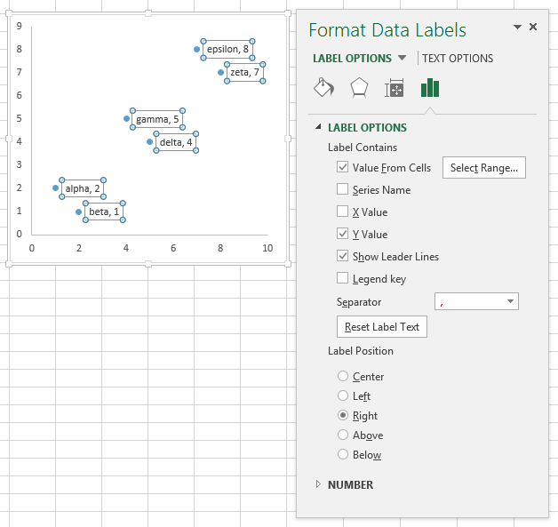
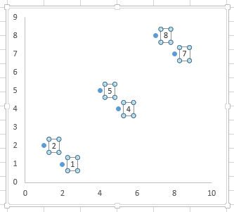
Improve your X Y Scatter Chart with custom data labels

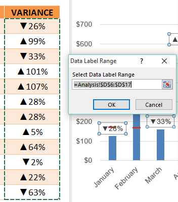
Excel Tips n Tricks -Tip 8 (Applying Chart Data Labels From a Range in ... Click on the plus symbol, the first icon, and check "Data Labels". Now you will see them added to your chart. You can also click on the right arrow on "Data Labels" and select where you want the data labels to be aligned, in other words center, right, top, bottom and so on. Picture 4, 4. I modified the chart and axis titles to look good.

Change the format of data labels in a chart

Format Data Labels in Excel- Instructions - TeachUcomp, Inc. To format data labels in Excel, choose the set of data labels to format. To do this, click the "Format" tab within the "Chart Tools" contextual tab in the Ribbon. Then select the data labels to format from the "Chart Elements" drop-down in the "Current Selection" button group.

Adding rich data labels to charts in Excel 2013 | Microsoft ...

Excel 2013 - Line Chart Data Labels - Data Callout submenu missing In one of them I can see the Data Callout submenu which allows me to specific content for data labels to appear at specific points on the line-graph. The "label options/label contains" area in the formatting box then includes a "value from cells" tickbox that allows me specify that the values that come from a specific excel cell range.

Apply Custom Data Labels to Charted Points - Peltier Tech

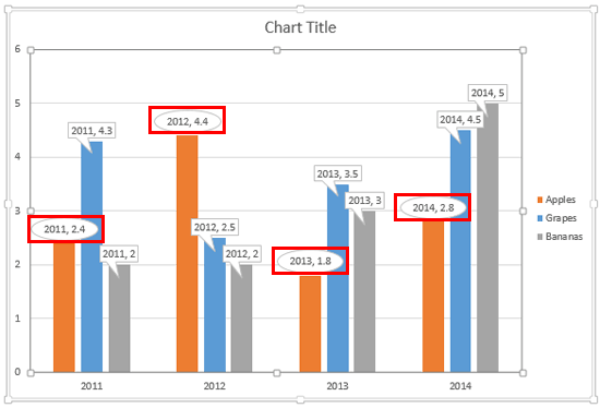
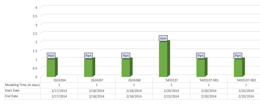
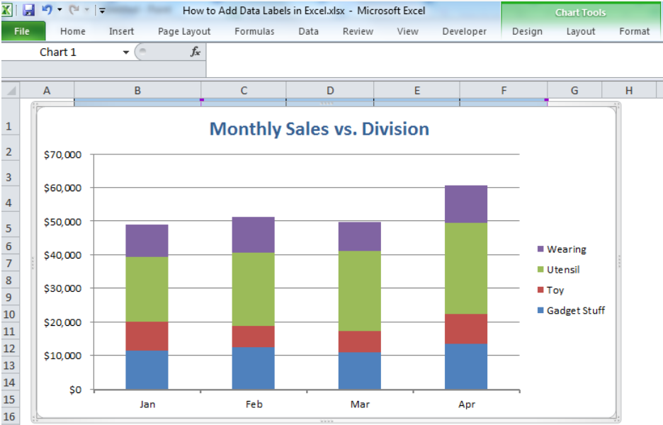
How to Add Data Labels to your Excel Chart in Excel 2013 Data labels show the values next to the corresponding chart element, for instance a percentage next to a piece from a pie chart, or a total value next to a column in a column chart. You can choose...

Excel charts: add title, customize chart axis, legend and ...

Adding rich data labels to charts in Excel 2013 - Microsoft Excel 2013 also lets you put numbers from your spreadsheet into your data labels - that is, numbers that are not directly associated with the data point. Here is a quick example. Let's say that I want to add a further annotation about the temperature on Wednesday and I want to include a data value with that annotation. Here's how I would do it:

How to Add Data Labels in Excel - Excelchat | Excelchat

Data Labels in Excel Pivot Chart (Detailed Analysis) 7 Suitable Examples with Data Labels in Excel Pivot Chart Considering All Factors, 1. Adding Data Labels in Pivot Chart, 2. Set Cell Values as Data Labels, 3. Showing Percentages as Data Labels, 4. Changing Appearance of Pivot Chart Labels, 5. Changing Background of Data Labels, 6. Dynamic Pivot Chart Data Labels with Slicers, 7.

Apply Custom Data Labels to Charted Points - Peltier Tech

Excel 2013 Graphs automatically aligning data labels to end of bar Excel 2013 Graphs automatically aligning data labels to end of bar, Hi, In Excel 2013 I am wanting to align the data labels in a graph automatically to be at the end of the bar (in a bar graph obviously). I know how to move them manually, but I remember there used to be a way to make it move them all automatically.